Introduction
In this blogpost I describe the history of z9, our detection engine. I will show its performance over reference data sets commonly used in the machine learning community. I’ll then describe how we apply it to detect networks attacks without any type of packet inspection.
Eventually, we encourage you to participate by helping us gather and validate performance data from your own enterprise-grade network IPS. This data will be compared with our mobile device, non-intrusive zero-packet technique compiled and published here as part of our blogpost series alongside our documented research paper release.
I would like to thank @ihackbanme for the strong belief in the data model prediction accuracy over the years (since 2012) ,@zesteban for the sisyphean yet phenomenal job of implementing all the optimization algorithms required and tweaking the classifiers to create our award-wining detection engine, @chiconara who works hard in keeping z9 fit for various complex data models and helping us win cyber security machine learning (CSML) competitions. And our newest zLabs team member @federicopomar.
What is Zero Packet Inspection?
Modern computing devices such as tablets, smartphones and other wearable devices are not architecturally designed to comply with security standards and permission models which do not allow generic user mode detection capabilities based on packet inspection.
Zero Packet Inspection, ZPI, uses the statistics collected in realtime over the operating system’s network stack without intervening or monitoring of the actual packets or traffic. ZPI not only reduces the amount and density of data that needs to be processed and inherently the number of CPU cycles needed to be spent, it also increases the discrimination of end-cases resulting in fewer false positives and better capabilities to correlate better despite various end-case scenarios.
In 2015, the USPTO granted our patent, two years after we filed our first provisional, describing our usermode detection capabilities. @zesteban has completed the commercialization process of z9 engine where our models worked perfectly for iOS/mac OS X and Android/Linux platforms. Recently, it was validated by @chiconara that these models were also suitable for the Windows platform.
What is the z9 engine?
In January 2013, we introduced the first user mode classifier portraying a multiclass model which can detect most types of network scans and MITM without any packet analysis. It was mostly based upon statistical SNMP and route information associated with the different protocols and network interfaces. It was a breakthrough in the detection capabilities known at the time. As a result, we were able to prove that our detection was a strong rival to deep packet inspection of high-end next generation enterprise IPS’s.
Over the years, z9 detection capabilities were extensively tested in the field over the Android and iOS platforms. z9 gave us the perfect toolset to further detect on different vectors and different datasets such as host operating system detection, gaining us the capability to detect sophisticated attacks such as Stagefright and Rowhammer.
As a result, we created an immense advantage using this technique, since we have the ability to maintain user privacy while detecting attacks that enterprise appliances find hard to cope with literally fractions of the resources.
Generalized Benchmarks
In order for us to benchmark our engine against commercial classifiers and find innovative ways to creatively outperform state-of-the-art classifiers over generic UCI and Kaggle datasets, we used several metrics described below.
To measure the quality of a classifier, each dataset was split in two smaller sets: 70% to train the classifier (training set) and 30% to test how well it performs over new, unseen data (test set). The test classification error was used as the accuracy of the classifier (the lower the error, the more accurate the classification).
Results of these confusion matrices are shown for z9 against other available classifiers in the industry (Table 1). The method best fit for the training sets are shown in gray, and the best method for the test sets in green. The complete paper will describe the full confusion matrices and the winnowing, outliers, de-noising process we use pre-classification.
|
Classification Error [%] |
||||||||||||
|
Data Set |
z9 |
|||||||||||
| Train | Test | Train | Test | Train | Test | Train | Test | Train | Test | Train | Test | |
| Letters | 0.00 | 2.56 | 23.5 | 23.7 | 0.57 | 2.56 | 4.00 | 12.50 | 0.03 | 4.90 | 0.00 | 4.28 |
| Optdigits | 0.00 | 2.39 | 0.00 | 6.00 | 3.16 | 3.51 | 2.10 | 13.70 | 0.00 | 5.80 | 0.00 | 2.95 |
| pendigits | 0.00 | 2.34 | 4.10 | 9.40 | 0.63 | 4.54 | 9.00 | 7.70 | 0.02 | 4.30 | 0.00 | 3.60 |
| satimage | 0.00 | 8.95 | 18.40 | 20.80 | 9.85 | 14.65 | 3.40 | 14.20 | 0.00 | 10.30 | 0.00 | 8.98 |
| segment | 0.00 | 2.86 | 3.10 | 6.10 | 2.53 | 4.42 | 0.60 | 6.00 | 0.10 | 4.90 | 0.00 | 3.25 |
| vehicle | 0.00 | 24.47 | 19.50 | 25.60 | 7.82 | 24.47 | 4.60 | 33.00 | 0.00 | 28.4 | 0.00 | 29.43 |
| waveform-21 | 0.00 | 17.36 | 8.40 | 17.70 | 6.33 | 19.11 | 2.70 | 29.70 | 0.00 | 21.3 | 0.00 | 17.38 |
| wine | 0.00 | 0.00 | 0.00 | 5.10 | 0.00 | 1.67 | 0.80 | 15.00 | 0.00 | 10.00 | 0.00 | 3.33 |
| creditcardfraud | 0.00 | 0.05 | 0.15 | 0.17 | 0.09 | 0.11 | 0.09 | 0.13 | 0.04 | 0.07 | 0.01 | 0.05 |
| hr-analytics | 0.06 | 1.09 | 18.36 | 17.72 | N/A | N/A | 1.78 | 2.29 | 1.50 | 2.02 | 0.03 | 0.85 |
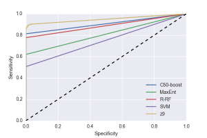
Another commonly used metric is the Receiver Operating Characteristic (ROC) curve, which shows how fit a classifier is to a given problem (see Fig. 1).
The two axes represent the tradeoffs between errors (false positives) and accurate predictions (true positives) a classifier makes. The resulting performance can be graphed in two dimensions, which is easy to visualize.
The AUC (area under the curve) is a measure of the discriminability of a pair of classes. In a two-class problem, the AUC is a single scalar value, yet a multiclass problem introduces the issue of combining multiple discriminations.
For the multiclass problems mentioned above,we chose Hand & Till AUC generalization and compiled the results for the datasets mentioned above ( See Table 2).
Figure 1 ROC curves for the different classifiers used for the creditcardfraud dataset
|
AUC (AREA UNDER CURVE) |
|||||
|
C50 boosted |
R-RF |
zee9 |
Max Entropy |
LibSvm |
|
| letter | 0.9996 | 0.9999 | 0.9995 | 0.7666 | 0.9968 |
| optdigits | 0.9930 | 0.9905 | 0.9997 | 0.7713 | 0.6667 |
| pendigits | 0.9975 | 0.9963 | 0.9993 | 0.8978 | 0.7777 |
| satimage | 0.9966 | 0.9976 | 0.9932 | 0.9288 | 0.7303 |
| segment | 0.9979 | 0.9978 | 0.9993 | 0.9042 | 0.9996 |
| vehicle | 0.9134 | 0.9033 | 0.9270 | 0.8798 | 0.5001 |
| waveform-21 | 0.9022 | 0.8721 | 0.9715 | 0.7350 | 0.6623 |
| wine | 0.9046 | 0.9872 | 1.0000 | 0.8646 | 0.6674 |
| creditcardfraud | 0.9065 | 0.8850 | 0.9961 | 0.8098 | 0.7530 |
| hr-analytics | 0.963066 | 0.9806 | 0.9923 | 0.7028 |
N/A |
Table 2. AUC for the classifiers on MC datasets benchmarked.
Zero Toxicity?
Previously published experimental studies described port scans combined with vulnerability scans as a relevant indicator of an upcoming attack, yet reconnaissance severity from network risk perspective is considered low and due to its complexity is being largely ignored as a risk factor.
To illustrate the complexity, consider a streaming or chat application, it would need to hole-punch connections for a legitimate p2p streaming using conventional Interactive Connectivity Establishment ( ICE ) or performing similar naive network operations. If you would try to pick up UDP scans from Packet filtering analysis or DPI, it would be hard to distinguish them from the ‘hole-punching’ candidate selection process. It would not justify the resources required for by the DPI mechanism and will fail on fragmented or time window independent variations of the scan. This problem must be solved with very high accuracy and very low false positive rate due to the base rate fallacy.
Portability of Zero Packet Inspection
Although the contextual and associative weight of the features across operating systems is somewhat similar, suggesting some normalization can be performed; different methods however are obviously used to collect the features. As the collection process itself may with some extent be affected by the operating system scheduler, memory allocation and paging strategy. As well as other operating system internal traits, indirectly affecting the network stack. It is important to decouple any influence done by the sampling process, to ensure the correlation is not subjected to the sampling time window or other traits subjected to this specific device architecture which may influence time series in that manner.
Paper Release Schedule
As a symbolic tribute to John Henry Holland, we would like to share and publish our benchmarking white paper describing the network detection capabilities across multiple operating systems (XNU, linux or Windows based) on Aug. 9. 2017 in memory of one of the people who inspired our team and our engine.
Call for Participation / Contribution
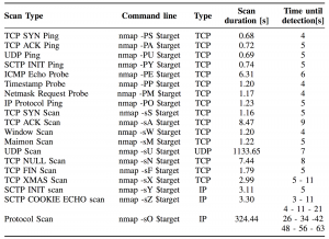
We encourage research and academic institutes, as well as professional enterprise IT readers, to participate and contribute to our post accompanying the white paper by running the following NMAP commands and collecting the result values as described on table 3:
Table 3. Example of scan time window detection. With -T3 flag for scan time windows. Multiple detection are listed as multiple times ( tested on Samsung Galaxy S6 Android 6.0)
Supplementary to the efficacy of the current solution, we would like to measure and compare the sensitivity of the detection given various time windows as illustrated on the table above, the precision of the detection is rounded to seconds for simplicity.
To contribute , please send us your results to signal@zmpr.co
Part II of ZPI published here:
https://blog.zimperium.com/zpi-one-approach-rule/
References:
M.H. Bhuyan,D. Bhattacharyya, and J.K. Kalita, “Surveying port scans and their detection methodologies,” The Computer Journal, p. bxr035, 2011.
Panjwani, S., Tan, S., Jarrin, K. M., & Cukier, M. (2005, June). An experimental evaluation to determine if port scans are precursors to an attack. In Dependable Systems and Networks, 2005. DSN 2005. Proceedings. International Conference on (pp. 602-611). IEEE.
- W. Frey and D. J. Slate (Machine Learning Vol 6 #2 March 91): “Letter Recognition Using Holland-style Adaptive Classifiers”.
- Kaynak (1995) “Methods of Combining Multiple Classifiers and Their Applications to Handwritten Digit Recognition”
F.Alimoglu (1996) Combining Multiple classifiers for pen-based Handwritten digit recognition”
Feng,C., Sutherland,A., King,S., Muggleton,S. & Henery,R..(1993). Comparison of Machine Learning Classifiers to Statistics and Neural Networks.
- Zupan, M. Bohanec, I. Bratko, J. Demsar: Machine learning by function decomposition. ICML-97, Nashville, TN. 1997
- Bohanec and V. Rajkovic: Knowledge acquisition and explanation for multi-attribute decision making. In 8th Intl Workshop on Expert Systems and their Applications, Avignon, France. pages 59-78, 1988.
Breiman,L., Friedman,J.H., Olshen,R.A., & Stone,C.J. (1984).
Classification and Regression Trees. Wadsworth International
Forina, M. et al, PARVUS – An Extendible Package for Data Exploration, Classification and Correlation. Institute of Pharmaceutical and Food Analysis and Technologies, Via Brigata Salerno
Breiman, L. Bagging Predictors Machine Learning, 1996, Volume 24, Number 2, Page 123
Breiman, L. RANDOM FORESTS Statistics Department University of California Berkeley, CA 94720 January 2001
Quinlan, J.R. (1979). Discovering rules by induction from large collections of examples. In D. Michie (Ed.), Expert systems in the micro electronic age. Edinburgh: Edinburgh University Press. Quinlan, J.R. (1986). Induction of decision trees. Machine Learning, 1, 81-106.
Holland, J.H., Holyoak, K.J., Nisbett, R.E., & Thagard, P.R. (1986). Induction: Processes of inference, learning, and discovery. Cambridge, MA: The MIT Press.
A Simple Generalization of the Area Under the ROC Curve for Multiple Class Classification Problems – David Hand and Robert Till (2001).


